Examples¶
Every script here is runnable from a clone, and every figure was written by the script beside it. Continuous integration regenerates them and fails the build if any differ.
A single layer, against the closed form¶
examples/01-single-layer.mjs
One quarter-wave layer on a substrate at normal incidence has an exact solution:
Macleod, Thin-Film Optical Filters 5th ed., §3.2. It is the simplest case where a transfer-matrix implementation can be checked against something that is not another transfer-matrix implementation.
quarter-wave thickness   99.6377 nm
R from tmmcore           0.012600790214630274
R closed form            0.012600790214630288
difference               1.39e-17
R + T + A                1.0000000000000000

bare glass R             4.26 %
coated R                 1.26 %
The disagreement is below double-precision epsilon.
An antireflection coating¶
examples/02-ar-coating.mjs
The classic quarter–half–quarter design: a quarter-wave of low index facing air, a half-wave of high index, a quarter-wave of intermediate index against the substrate. The half-wave layer is an absentee at the reference wavelength and flattens the response either side of it.
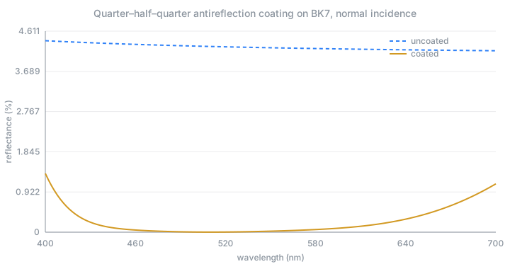
The dispersion functions are Cauchy-style approximations chosen to be representative. Real work uses measured n,k. tmmcore takes the index at the wavelength you are evaluating and has no opinion on where it came from.
A metal mirror at oblique incidence¶
examples/03-metal-mirror.mjs
Metals are where transfer-matrix implementations are most likely to diverge: k is large, the phase thickness is strongly complex, and the field decays within tens of nanometres. At 45° the s and p responses separate, and absorptance shows it most clearly.
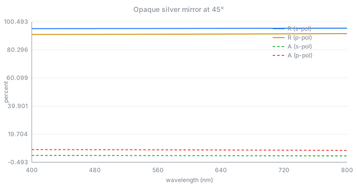
           Rs %     Rp %     As %     Ap %
400 nm   95.587   91.369   4.413   8.631
550 nm   95.665   91.518   4.335   8.482
700 nm   95.799   91.774   4.201   8.225

max transmittance through 120 nm of silver: 1.73e-6
"Opaque" is a judgement about a number, and how small the number needs to be depends on your design, so the example prints it rather than assuming it.
Wavelength against angle of incidence¶
examples/05-angle-map.mjs
A quarter-wave stack, (HL)⁸H with λ₀ = 700 nm, swept over 400–1000 nm and 0–80° in both polarizations.
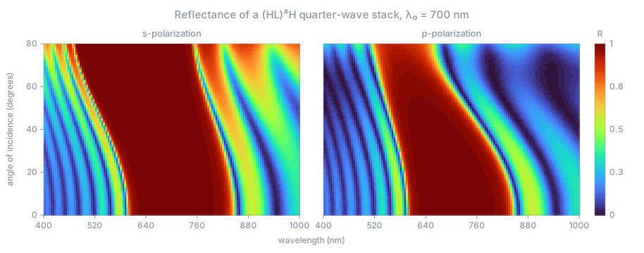
The high-reflectance zone bends toward shorter wavelengths as the stack is tilted. The phase thickness at oblique incidence is \(\delta = 2\pi n d \cos\theta / \lambda\), which reads as an apparent optical thickness \(nd\cos\theta\), so the layers behave as though they were thinner when tilted (Macleod, Thin-Film Optical Filters 5th ed., ch. 8, "Simple Tilts in Collimated Light"). For the quarter-wave stack specifically: "As the multilayer is tilted to greater angles of incidence, the characteristic moves to a shorter wavelength" (ch. 10, One-Dimensional Photonic Crystals).
R >= 0.9 band, nm
  AOI      s-pol           p-pol
   0°   605-830         605-830
  30°   575-810         590-785
  45°   540-785         570-730
  60°   505-765         555-675

s-pol band centre moves 83 nm to the blue between 0° and 60° (717.5 -> 635 nm).

reference points
   700 nm   0°  s   R = 0.999457736995
   550 nm   0°  s   R = 0.092532958768
   450 nm   0°  s   R = 0.049112277617
   700 nm  45°  s   R = 0.999740289709
   700 nm  45°  p   R = 0.988233906498
   600 nm  60°  s   R = 0.999971652485
   600 nm  60°  p   R = 0.987906648644
The two polarizations are identical at normal incidence and separate as the angle grows, with the p-polarized zone narrowing faster. Indices are non-dispersive here so that the tilt is the only effect in view, which also makes the design trivial to reproduce in another tool: air, then 17 alternating quarter waves starting and ending with H, on a substrate of index 1.52.
The reference points are point samples at full precision, so they can be checked against another implementation without depending on where a band edge happens to fall on the grid.
The figure itself averages R over each cell's wavelength bin. The sidelobe fringes on the short-wavelength side are narrower than one cell, and point sampling would alias them into speckle; the average is what a spectrophotometer of finite bandwidth measures.
Refinement with the analytic Jacobian¶
examples/04-refine.mjs
tmmThicknessJacobian returns \(\partial R/\partial d_j\) for every layer, exactly, from the same matrix product that produced \(R\). No other transfer-matrix package offers this.
The example starts from a deliberately poor guess and runs damped Gauss–Newton against a target of zero reflectance across the visible. Residuals are \(R(\lambda_i)\); Jacobian rows are \(\partial R(\lambda_i)/\partial d_j\).
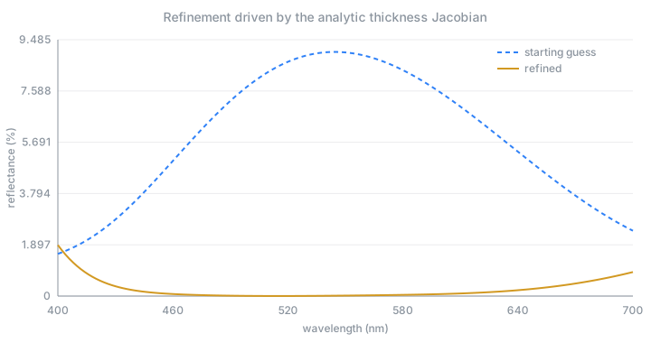
start        mean R = 6.6880 %   d = [70.00,150.00,40.00]
iteration  1  mean R = 2.9619 %   d = [70.43,125.94,107.89]
iteration  2  mean R = 0.8692 %   d = [87.68,129.27,96.63]
iteration  3  mean R = 0.4146 %   d = [93.12,125.63,86.82]
iteration 10  mean R = 0.2491 %   d = [93.64,114.88,72.62]
iteration 16  mean R = 0.2350 %   d = [93.35,117.34,74.56]

refined      mean R = 0.2348 %   d = [93.62,117.56,75.42]
The optimizer converges to [93.6, 117.6, 75.4] nm. The textbook quarter–half–quarter design for these materials is [92.4, 115.9, 75.0] nm.
A finite-difference Jacobian would need one extra spectrum evaluation per layer per iteration. Here the derivatives arrive with the spectrum. For a three-layer stack that is a factor of four; for a forty-layer stack it is a factor of forty-one.
The needle P-function: where the next layer goes¶
examples/06-needle.mjs
tmmNeedleScan returns the derivative of each spectral quantity with respect to inserting an infinitesimally thin layer of a candidate material, at every position in the stack at once. Chain that through a merit function and you get P(z), whose most negative point is the best place to insert.
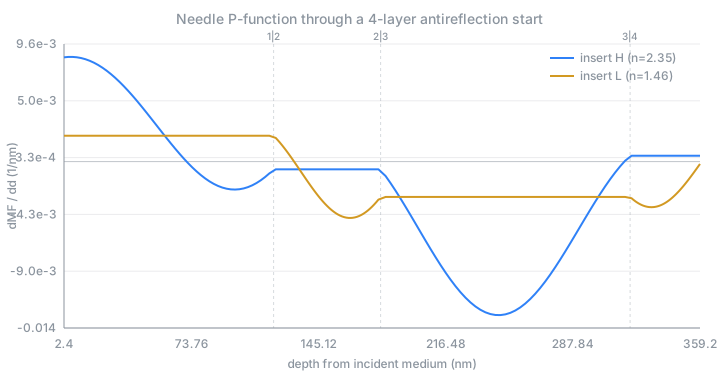
Starting from a deliberately mediocre four-layer antireflection design, with mean R² over 450–650 nm as the merit function:
start design, 4 layers, 360 nm total
merit (mean R^2 over 450-650 nm) = 1.1956e-1

most negative P: -1.2562e-2 /nm
  candidate H (n=2.35) at depth 247.2 nm from the incident medium
P is the \(d \to 0\) limit of Sullivan and Dobrowolski's numerical pre/post method (Appl. Opt. 35, 5484, 1996), the analytic P-function of Tikhonravov et al. (Appl. Opt. 35, 5493, 1996). Unlike the numerical form it needs no trial thickness and no second spectrum evaluation.
Being a limit, it is checkable. Insert a needle of thickness \(\varepsilon\) at that point and the numerical slope has to converge to it:
   eps (nm)   (MF(eps) - MF(0)) / eps        ratio to analytic
   1          -1.221337e-2              0.972233
   0.1        -1.252856e-2              0.997324
   0.01       -1.255883e-2              0.999734
   0.001      -1.256184e-2              0.999973
Which layer controls which wavelength¶
examples/07-jacobian-map.mjs
tmmThicknessJacobian returns R and \(\partial R/\partial d_j\) for every layer. Evaluating it at each wavelength gives a signed sensitivity map of the quarter-wave reflector from the angle example, with one row per layer and one column per wavelength.
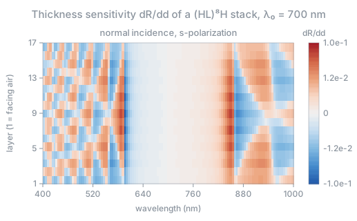
largest |dR/dd| over the grid: 9.9781e-2 /nm

peak |dR/dd| inside the 620-800 nm zone : 6.5219e-4 /nm
peak |dR/dd| anywhere on the grid       : 9.9781e-2 /nm
ratio                                   : 153.0x
Deep inside the high-reflectance zone R is pinned near 1, so no layer can move it and the map goes neutral. All the leverage sits at the band edges and in the sidelobes, which is why refining a reflector means working on its edges.
The colour scale is a signed cube root. Those two band edges carry derivatives 150 times larger than anything else, and on a linear scale 87% of the map renders as blank neutral; the cube root keeps the sign, compresses the peaks and opens up the sidelobe structure. The colour bar is labelled accordingly.
Verified against a central difference at a band edge, where the derivative is largest:
analytic dR/dd against a central difference at 615 nm, h = 1e-4 nm
  layer    analytic          central diff      rel. difference
      1    -4.932399e-4    -4.932399e-4    4.9e-9
      5    -1.191639e-3    -1.191639e-3    9.9e-10
      9    -1.366824e-3    -1.366824e-3    2.6e-9
     17    -3.083978e-4    -3.083978e-4    8.4e-9
Group delay, against a closed form¶
examples/08-group-delay.mjs
A slab whose surrounding media share its own index has no interfaces, so nothing reflects and the transmission coefficient is a pure phase. Group delay, GDD and TOD then reduce exactly to bulk propagation, which gives a check on the phase kernel that does not go through another transfer-matrix calculation.
matched slab, 1 µm of n(λ) = 1.45 + 3600/λ², at 800 nm

            tmmcore            closed form         relative
  GD       4.89296832143789     4.89296832143789   1.8e-16  fs
  GDD    0.0478126142151489   0.0478126142151501   2.6e-14  fs²
  TOD    0.0203063517881787   0.0203063517881746   2.0e-13  fs³
The example also builds the index jet the way you would in your own code, by composing a Cauchy formula through the jet arithmetic rather than differentiating it by hand.
The second half reads GDD off a chirped mirror and ranks its layers by \(\partial\mathrm{GDD}/\partial d\), which arrives in the same call:
24-layer chirped mirror, normal incidence

   λ (nm)      R        GD (fs)   GDD (fs²)   TOD (fs³)
     700  0.7330       2.03       87.0       -2839
     750  0.9708       1.80       11.7         -80
     800  0.9994       1.71       -0.3          31
     850  0.9999       2.04       -5.0          52
     900  0.9997       3.35      -21.0         307
Negative GDD across the design band is the point of a chirped mirror: the layer thicknesses ramp along the stack, so red turns around deeper than blue and comes back later, which is what compresses a pulse.
Where to go next¶
- API reference, every function and what it returns
- Validation, reproducing the accuracy figures yourself
- The needle P-function,
tmmNeedleScan, extends the idea above from optimizing thicknesses to deciding where a new layer should go. That is the basis of needle synthesis; TFStudio builds a full design environment on it.